Particle Swarm Optimization: Python Tutorial

Particle Swarm Optimization is one of the most successful and famous population-based metaheuristics. Its simplicity and performance made it easy to be adapted and used in many applications including the tasks of scheduling (more details can be found in my paper— Cloudlet Scheduling with Particle Swarm Optimization) or power consumption optimization in IoT devices (more details can be found in my paper— Particle Swarm Optimized Power Consumption Of Trilateration)

There are many versions of PSO such as the hybrid ones where PSO is used along with other algorithms (such as Simulated Annealing) in my publication above. But in general, when we are talking about a pure PSO algorithm we would recognize it as being a single or multi-objective that operates on a discrete or continuous space. The objectives of the algorithm are the things that PSO try to find a solution for. For example, PSO might concentrate on reducing the power consumption of a device without taking into consideration anything else, like the speed of the device. That’s why we developed multi-objective versions to kind of try to balance the solution. Balancing the work of the algorithm to consider more than one objective is part of the Game theory field (if you are curious and want to know more look at Nash Equilibrium and Pareto Optimality).

The original algorithm work on a continuous space. What that means is that it works to solve problems such as the numeric minimization problem I mentioned in the previous Heuristics post. PSO also works on a discrete binary space, which means that the algorithm is used to find a $ 0 $ or $ 1 $ values for the given problem (a simple example can be found in my scheduling paper). But now, let’s go back to our simple minimization problem and try to solve it using PSO. At this point if you didn’t read my other blog post please do so to know what I am trying to solve here.

PSO starts by creating a swarm of particles where each particle is a possible solution to the problem. Therefore, we need to understand what exactly we are trying to solve and how to map it to the objective function of PSO, which is considered the hardest part when designing the algorithm.

Let’s first define few global variables needed throughout our program

# the x and y in our function (x - y + 7) (aka. dimensions)
number_of_variables = 2
# the minimum possible value x or y can take
min_value = -100
# the maximum possible value x or y can take
max_value = 100  
# the number of particles in the swarm
number_of_particles = 10
# number of times the algorithm moves each particle in the problem space
number_of_iterations = 2000

w = 0.729 # inertia weight
c1 = 1.49 # cognitive (particle)
c2 = 1.49 # social (swarm)

The first step is to create the swarm of particles

swarm = [Particle(number_of_variables, min_value, max_value)
            for __x in range(number_of_particles)]

Where each Particle is an Abstract Data Type (ADT) defined as follows:

class Particle:

  def __init__(self, number_of_variables, min_value, max_value):

        # init x and y values
        self.positions = [0.0 for v in range(number_of_variables)]
        # init velocities of x and y
        self.velocities = [0.0 for v in range(number_of_variables)]

        for v in range(number_of_variables):
            # update x and y positions
            self.positions[v] = ((max_value - min_value)
                                    * random.random() + min_value)
            # update x and y velocities
            self.velocities[v] = ((max_value - min_value)
                                    * random.random() + min_value)

        # current fitness after updating the x and y values
        self.fitness = Fitness(self.positions)
        # the current particle positions as the best fitness found yet
        self.best_particle_positions = list(self.positions)
        # the current particle fitness as the best fitness found yet
        self.best_particle_fitness = self.fitness

Before I explain what each line means I should first explain how a particle behaves in the problem space then get back to our code snippet above.

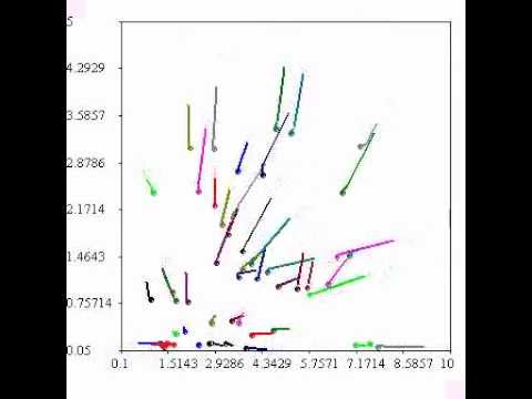
As I mentioned before, each particle in the swarm represents a possible solution to the problem. And as I also mentioned in the previous blog post, each particle try to improve its solution by learning from two sources: its movement in the problem space and the movement of the other particles of the swarm (through learning from the best solution found by any of the other particles). To watch a simple visualization of PSO click on the image below:

Now, let’s see how that translates into code. The positions list in the above code snippet represent the current values of the variables in the objective function ($ x $ and $ y $) where the velocities list represent the (artificial) velocities (for each position) of the particle in space. We first initialize the values to zeros then update them using random numbers as follows:

(( max_value - min_value) * random.random() +  min_value )

Each particle in our swarm keep track of its fitness value and the best positions and fitness found by any particle of the swarm (including itself). Where a particle fitness is the solution it achieved by plugging the current positions list values in the objective function (in our example problem, $ positions[0] = x $ and $ positions[1] = y $). Notice that during initialization we consider the particle’s fitness and positions as the best ones found yet because it might be the case, later we will check that and update with the correct information during each iteration of the algorithm.

After the initialization of the swarm, we check all particles and find the best solution found and keep track of that using the two variables best_swarm_positions and best_swarm_fitness.

best_swarm_positions = [0.0 for v in range(number_of_variables)]
best_swarm_fitness = sys.float_info.max

for particle in swarm: # check each particle
    if particle.fitness < best_swarm_fitness:
        best_swarm_fitness = particle.fitness
        best_swarm_positions = list(particle.positions)

Now, we are ready to start moving particles in the problem space by generating new velocities to find new positions ($x$ and $y$ values) and eventually find new solutions (fitness values). The fitness value of each particle in the swarm is going to be updated during each iteration of the algorithm.

for __x in range(number_of_iterations):
    for particle in swarm:
        # start moving/updating particles to calculate new fitness

Then, inside the nested loops, we start updating the velocities and positions and calculate the new fitness while keeping track of the best fitness of the swarm. But first, let’s start by updating the velocities as follows:

# compute new velocities for each particle
for v in range(number_of_variables):
    particle.velocities[v] = calculate_new_velocity_value(particle, v)

For each variable in the objective function, we should calculate a new velocity to later aid in calculating a new set of positions. That is done by calling calculate_new_velocity_value() function and passing the current particle and the variable number to it as follows:

# calculate a new velocity for one variable
def calculate_new_velocity_value(p, v):

    # generate random numbers
    r1 = random.random()
    r2 = random.random()

    # the learning rate part
    part_1 = (w * p.velocities[v])
    # the cognitive part - learning from itself
    part_2 = (c1 * r1 *
                  (p.best_particle_positions[v] - p.positions[v]))
    # the social part - learning from others
    part_3 = (c2 * r2 *
                  (best_swarm_positions[v] - p.positions[v]))

    new_velocity = part_1 + part_2 + part_3

    return new_velocity

As shown in the above code snippet, the value of the new velocity is the sum of all of the following three parts:

The learning rate part:

• The multiplication result of the inertia weight parameter ($w$) and the particle’s current velocity.
• The inertia weight parameter influences the convergence of the algorithm and the exploration of its particles. Therefore, a well-defined inertia weight is very important in influencing the quality of the solution found by PSO. The higher the inertia weight means bigger steps in the problem space (in other words, higher velocities). There are many types of inertia weights but we use in this example the fixed inertia weight (a static value) which do not change throughout the iterations. To learn more about other kinds of inertia weights read section 2.3.4 in my master thesis. Also, check how I used the simulated annealing and how it helped PSO in achieving better results in my paper (Cloudlet Scheduling with Particle Swarm Optimization).

The cognitive part:

• This part of the equation is the multiplication result of the constant c1 and the random number r1 and the subtraction of the position value that corresponds to the best fitness found by the particle and the current position value.
• The overall idea of this part of the equation is to represent the cognitive (self-learning) part of the particle.

The social part:

• The multiplication result of the constant c2 and the random number r2 and the subtraction of the position value that corresponds to the best fitness found by any particle of the swarm and the current position value of the particle.
• The overall idea of this part of the equation is to represent the social ability of the particle (learning from the swarm).

To keep our velocities within our desired range we use the following few lines of code:

if particle.velocities[v] < min_value:
    particle.velocities[v] = min_value
elif particle.velocities[v] > max_value:
    particle.velocities[v] = max_value

Now, we are ready to calculate our new positions values using our new velocities to later calculate the new fitness of each particle.

# compute new positions using the new velocities
for v in range(number_of_variables):
    particle.positions[v] += particle.velocities[v]

And again, to keep the values of the positions within control we use the following lines of code as before:

if particle.positions[v] < min_value:
    particle.positions[v] = min_value
elif particle.positions[v] > max_value:
    particle.positions[v] = max_value

Finally, we are ready to calculate the new fitness value using the objective function. As apparent in the following code snippet, we plug the two positions values in the objective function which corresponds to the $ x $ and $ y $ value in the original equation $ x-y+7 $.

# compute the fitness of the new positions
particle.fitness = Fitness(particle.positions)

def Fitness(positions):
    #                 x -            y + 7
    return positions[0] - positions[1] + 7

At the end of each iteration, we evaluate the quality of the newly calculated fitness value and use it to do two kinds of updates if it is of a high quality. The first is to update the value of the best fitness found by the particle we are moving and the second is to update the value of the best fitness found by any particle of the swarm. Remember that the whole point of using PSO is to find the values of $ x $ and $ y $ such that we minimize the value of the whole function. Therefore, the best solution to the problem would be $ -100 - +100 + 7 $ which equals to $ -193 $ and PSO would be able to find the correct solution by the end of the iterations.

You can also download the full code and play with it yourself. And with that, I finish this post. I hope you learned something new and if you have any question don’t hesitate to contact me. Happy learning!